Critical length revisited: how long should ONT reads be for structural variant discovery?
Wouter De Coster
structural variantsread lengthOxford NanoporeSniffles2benchmarking
1716 Words · 7 Minutes, 48 Seconds
2026-10-31 08:00
In 2020 we published Critical length in long-read resequencing, in which we simulated reads of a fixed length from human genome assemblies and concluded that reads of about 20 kb are sufficient for structural variant (SV) discovery. Six years later, both the data and the tools have changed, so I revisited the question.
The short answer: the 2020 ballpark holds, but now as a library N50 rather than a fixed read length. For SV discovery from ONT R10 reads, a library with a read N50 of 20–30 kb gets you within a few F1 points of what much longer reads give. The variants that keep benefiting from longer reads are insertions of more than 1 kb and SVs in long, near-identical segmental duplications, where an ultra-long library still helps. Going from 15x to 30x gains about as much as going from a 20 kb to a 100 kb N50.
What is different from 2020
| 2020 | Now | |
|---|---|---|
| Reads | Simulated (SimLoRD, a PacBio error model in which short fragments are read in several passes and are therefore more accurate) | Real ONT R10.4.1 reads, cut to length |
| Read lengths | One fixed length per dataset | Fixed lengths, and the read length distribution of real libraries rescaled to a range of N50 values |
| Genome and truth set | HG00733 (and CHM13 draft, NA12878): SVs called from its own assembly | HG002, with the GIAB v5.0q SV benchmark built from the near-complete HG002 Q100 assembly |
| Software | minimap2 2.14, Sniffles 1.0.10, SURVIVOR matching (same type, breakpoints within 500 bp) | minimap2 2.31, Sniffles2 2.8.1, truvari 5.5.0 |
| Evaluation | Genome-wide, unstratified | Stratified by SV type, size and genomic context (tandem repeats, segmental duplications, low mappability) |
| Coverage | 40x (and 20x) | 15x and 30x |
The two changes that matter most are the reads and the length distribution. Simulated reads only came from assembled sequence, and their accuracy changed with their length, as it did for PacBio data at the time but does not for ONT, so read length and accuracy could not be separated. Real nanopore reads keep their real error profile at every length. A single fixed length per dataset is also not what a sequencing run produces.
Approach
All code is available at github.com/wdecoster/critical-length-revisited.
I used the public ONT HG002 ultra-long R10.4.1 data (sup basecalling, two flow cells, 53x coverage, read N50 of 106 kb, and 16x in reads of at least 150 kb).
- Fixed length: every read of at least L is cut into pieces of exactly L, placed at random within the read, for L from 1 to 150 kb.
- Library N50: pieces are drawn from the read length distribution of a standard ONT HG002 library (the public
giab_2025.01data, ligation kit), rescaled to an N50 of 5 to 100 kb. This is closer to what you actually get from a sequencing run than a single length.
The pieces were aligned with minimap2, subsampled to 15x and 30x, and SVs were called with Sniffles2 and compared to the GIAB HG002 v5.0q benchmark on five chromosomes, split by SV type, size and genomic context.
The details
- Long pieces only fit in long reads, so the drawing is calibrated until the pieces’ N50 is within 1% of the target.
- Alignment with minimap2 (
lr:hq) to GRCh38 (no-alt analysis set), subsampled to exactly 15x and 30x in the evaluation regions. - Chromosomes chr1, chr7, chr15, chr16 and chr20 (about 20% of the genome, 6,176 benchmark SVs, 555 of them in segmental duplications). The segmental duplication partners of these chromosomes elsewhere in the genome are included, so that reads from paralogous copies can still mismap into them.
- Genomic context from the GIAB v3.6 stratifications: tandem repeats, segmental duplications, low mappability and the rest.
- Scoring uses GIAB’s benchmarking setup for truvari: matching on position, size and sequence, followed by
truvari refine, which realigns the calls and the benchmark locally where they disagree (mostly in tandem repeats, where the same SV can be represented in different ways). Without sequence comparison and refine, the F1 values are 0.02–0.03 lower, with the same shapes.
Results
Library N50
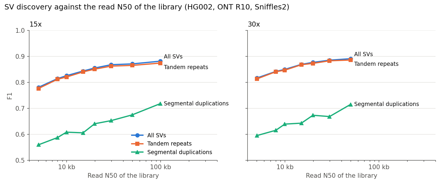
| Library N50 | All SVs, 15x | All SVs, 30x | Segmental duplications, 15x | Segmental duplications, 30x |
|---|---|---|---|---|
| 5 kb | 0.781 | 0.816 | 0.559 | 0.595 |
| 8 kb | 0.814 | 0.842 | 0.587 | 0.615 |
| 10 kb | 0.825 | 0.849 | 0.608 | 0.639 |
| 15 kb | 0.843 | 0.869 | 0.605 | 0.642 |
| 20 kb | 0.855 | 0.876 | 0.640 | 0.673 |
| 30 kb | 0.868 | 0.885 | 0.652 | 0.668 |
| 50 kb | 0.871 | 0.891 | 0.674 | 0.715 |
| 100 kb | 0.881 | – | 0.718 | – |
F1 (Sniffles2, GIAB truvari setup with refine) by library N50 and coverage. The ultra-long data do not have enough coverage for 30x at a 100 kb N50.
The F1 rises steeply up to an N50 of about 20 kb and gains only about 0.03 from 20 to 100 kb. Doubling the coverage to 30x shifts the whole curve up by 0.02–0.035. Almost all of the gain is in recall: precision stays at 0.93–0.95 at every N50 and coverage. Variants in tandem repeats, two thirds of the SVs, follow the overall curve. Variants in segmental duplications are a different story: their F1 is much lower and still increasing at 100 kb.
The details
- The segmental duplication values are noisier (555 SVs) and not strictly increasing from one N50 to the next, but the trend from 0.61 at 10 kb to 0.72 at 100 kb (15x) is consistent at both coverages.
- The shape of the read length distribution matters little: the standard library’s distribution and the ultra-long library’s distribution, rescaled to the same N50, give F1 values within 0.02 of each other (the standard shape slightly ahead). The N50 is therefore a reasonable single number to plan with.
Fixed read length
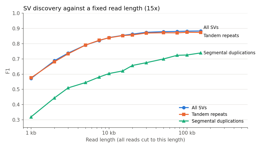
With all reads cut to the same length, the F1 plateaus at about 0.88 from 50 kb onward, and reads of 20–30 kb are within 0.01–0.02 of that. The difference between SV types is informative:
- Deletions: reads of 2–3 kb already find most of them.
- Insertions need reads of about 20 kb, because the read has to contain the inserted sequence and anchor on both sides.
- Insertions of more than 1 kb and segmental duplications keep improving up to 100 kb and beyond. Deletions of the same size do not need long reads.
The details
- Deletions: F1 0.84 at 3 kb, 0.87 at 10 kb, 0.88 at most.
- Insertions: 0.83 at 10 kb, 0.86 at 20 kb, 0.89 at most.
- Insertions of 1–6 kb: F1 0.72 with 10 kb reads, 0.83 at 20 kb and 0.91 at 100 kb; of 6–10 kb: 0.49, 0.75 and 0.88. Deletions of 1–6 kb are at 0.83 already with 2 kb reads (0.88 at 10 kb, 0.93 at 100 kb), and those of 6–10 kb at 0.95 with any length.
- SVs of more than 10 kb are rare in the benchmark (39 in these chromosomes) and are often missed even with 150 kb reads.
- Segmental duplications: F1 0.66 at 20 kb, 0.74 at 150 kb.
- Replicate cuts at 5, 20 and 100 kb gave F1 values within 0.005 of each other.
- Cutting the standard HG002 library to 10, 20 and 30 kb gave the same results as cutting the ultra-long library, so the ultra-long library does not behave differently once the length is fixed.
Then and now
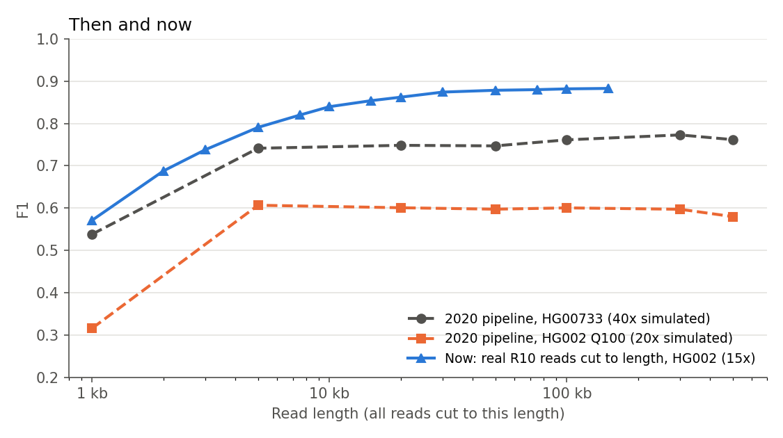
To place this next to the 2020 result, I reran the 2020 pipeline unchanged on the HG00733 assembly used in the paper, and on HG002 Q100.
Two things stand out. First, the simulated curves are flat from 5 kb (the first simulated length after 1 kb), while real reads keep improving up to 20–30 kb. Part of that difference comes from the simulation: SimLoRD models PacBio sequencing, in which a short fragment is read in several passes and is therefore more accurate than a long one, while ONT reads have the same accuracy at every length. Second, the small decline at the longest simulated lengths that we reported in 2020 also appears with the gap-free HG002 Q100 assembly, so it is not caused by assembly gaps. Real reads show no decline up to 150 kb, the longest length with enough coverage, so I would not plan around it.
The details
- The 2020 pipeline: SimLoRD simulation, minimap2 2.14, Sniffles 1, SURVIVOR matching. It scores against its own assembly-based truth with looser matching, and the simulated curves are at 40x (HG00733) and 20x (HG002), against 15x for the real reads, so the absolute values are not directly comparable to the truvari-based curve.
- In the simulation, reads were only drawn from assembled sequence, which excluded the regions where length matters most, and the effect of length was partly offset by accuracy.
- The decline on HG002 Q100 is in recall: 0.49 at 100 kb, 0.45 at 500 kb, with precision going up (not plotted; the F1 drops from 0.60 to 0.58 between 300 and 500 kb).
Recommendation
- Aim for an N50 of 20–30 kb for SV discovery from ONT R10 reads. Beyond that the overall gains are small (about 0.03 F1 from 20 to 100 kb at 15x).
- Once you are there: Invest in coverage before read length, as 30x instead of 15x gains as much as going from a 20 kb to a 100 kb N50.
- Go ultra-long for insertions of more than 1 kb and segmental duplications, which keep improving with read length, or if you plan to assemble.
- Deletions are already well called with short reads, so read length matters mostly for insertions and larger variants.
Limitations
- One genome (HG002), five chromosomes, the GIAB benchmark regions only, and one SV caller, so the absolute F1 values are optimistic.
- Only read-based SV calling; assembly-based calling, phasing and the completeness of the inserted sequence are left for a follow-up.
The details
- The GIAB benchmark regions exclude the regions where alignment of the assembly to the reference breaks, which are among the hardest for read-based calling.
- Cut pieces lack the artifacts of real read ends (low-quality starts, adapter remnants), which slightly favours the shorter lengths.
Try it yourself
The cutting tool is standalone and part of the repository, if you want to repeat this for your own data or question:
# all reads cut to 20 kb
python workflow/scripts/cut_reads.py reads.fastq.gz --length 20000 --seed 1 --output pieces.fastq.gz
# pieces following a library's read length distribution, rescaled to an N50 of 20 kb
python workflow/scripts/cut_reads.py reads.fastq.gz --distribution lengths.tsv --n50 20000 --seed 1 --output pieces.fastq.gz
Feedback and suggestions are, as always, welcome.